Reproducible Applied Statistics: Is Tagging of Therapist-Patient Interactions Reliable?
K. Jarrod Millman, Kellie Ottoboni, Naomi A. P. Stark and Philip B. Stark
We are three applied statisticians (JM, KO, PS) at UC Berkeley working with a domain specialist (NS) at the University of Pennsylvania. Our case study involves assessing inter-rater reliability (IRR) of the assignment of “tags” applied by human raters to classify interactions during therapy sessions with children on the autistic spectrum.
An extended version of this case study along with the analysis script and results can be found at https://github.com/statlab/nsgk.
Workflow
 Our project arose from a pilot study NS was working on with Dr. Gilbert Kliman of the Children’s Psychological Health Center in San Francisco. To investigate therapeutic interventions with children on the autistic spectrum, Dr. Kliman and NS collected some observational data (described below). NS approached PS about the data and the problem NS was studying. After investigating the problem further, PS emailed JM and KO a one-page proposal for a stratified permutation test to assess inter-rater reliability using stratified samples. We (JM, KO, PS) had recently begun developing a general purpose Python package for permutation tests, called
 permute, based on our collaborations. PS suggested this would be an interesting example to include.
After coming to an initial understanding of NS’s underlying research question and experiment, including how she collected the data, we (JM, KO, PS) cleaned the data, developed a nonparametric approach to assessing IRR appropriate to the experiment, implemented the approach in Python, incorporated the resulting code into our evolving Python package of permutation tests, applied the approach to the cleaned data, documented the code and the analysis, and wrote up the results in LaTeX.
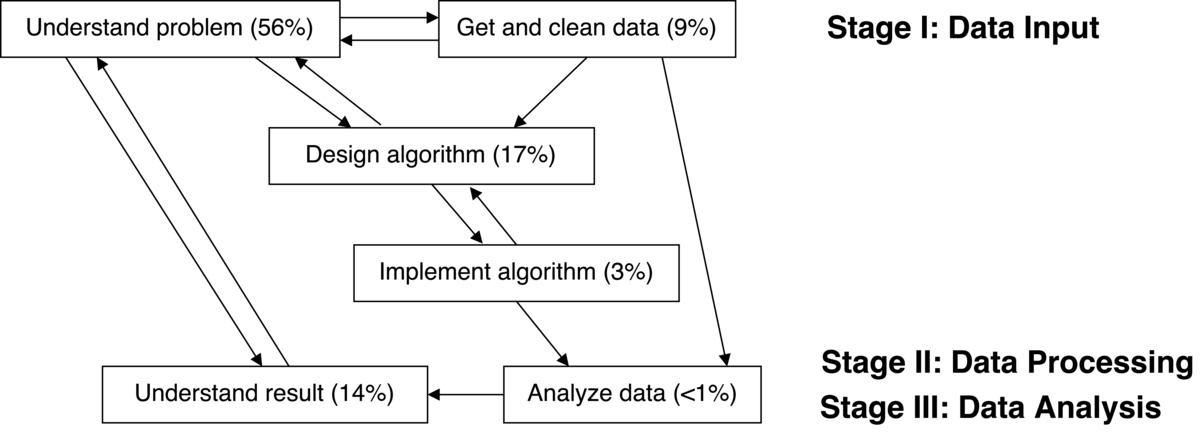
We distinguish the following aspects of our project, which are typical in applied statistics:
understand problem
get and clean data
design algorithm
implement algorithm
analyze data
understand result
Figure 1 shows how each aspect of the project influenced the other aspects and gives estimates of the total person-hours we collectively spent on each aspect of the project. For example, if JM, KO, and PS spent an hour together discussing the problem in a meeting, then that meeting counts as 3 people hours.
We did not keep a detailed record of time spent, but our computational practices provide enough detail about who did what when that we believe our estimates provide an accurate qualitative account of the time demands for each aspect of the project. However, since these are only rough estimates, the reader should focus on the relative differences in the amount of time we spent on each aspect. We have found that researchers (ourselves included) often underestimate the time needed to understand the problem, acquire and clean the data, as well as understand the results, while overestimating the time needed for writing code. We have included our time estimates to give people an idea how “inexpensive” (or expensive) working more reproducibly is, to capture how our group understanding evolved, and in the hope that it might be instructive for students and collaborators.
Since we view computational reproducibility as a cross-cutting concern of all project aspects, we have adopted a set of computational practices, which we (JM, KO, PS) followed (almost) whenever we were working on the project. Exceptions include that we did not record all of our in-person discussions or whiteboard work. However, we endeavored to record summaries of these activities. These computational practices, described in Millman & Pérez (2014), are used widely in the open source scientific Python community. While developed for managing software contributions, these practices are ideal for ensuring computational reproducibility in scientific and statistical research. We will illustrate how we leverage the software infrastructure and development practices of permute to conduct reproducible and collaborative applied statistics research with our colleagues. We discuss the software tools and practices briefly in Key tools and practices below.
Understand problem (80 hours)
The Kliman-Stark research project sought to identify characteristics of effective clinical interactions with children on the autistic spectrum. The project first required developing a set of characteristics that observers could use to “tag” what was happening in each 30-second interval of a therapy session. After they developed a taxonomy of clinical interactions, Kliman and NS had a number of trained raters watch videos of therapy sessions and label each 30-second interval using the collection of tags. For the classification system to be meaningful and useful, different raters must generally agree on whether a given tag applies to a given video segment: there must be inter-rater reliability. Of course, if a tag is never used or is always used, inter-rater reliability will be perfect, but the tag is useless for distinguishing clinical interactions.
That led to a statistical question: how to assess the evidence in the tagged videos that different raters tag interactions the same way? After numerous conversations, it made sense to consider the null hypothesis to be that, conditional on the number of times a given rater applied a given label to a given video, all assignments of that label to time stamps in the video by that rater are equally likely, and the ratings given by different raters are exchangeable (essentially, that raters are independent).
Once PS had an initial understanding of NS’s problem, we (JM, KO, PS) met regularly (approximately weekly, sometimes more) as a team to discuss the project. Initially these discussions involved a lot of work on whiteboards and asking a lot of probing questions. This helped us develop a shared understanding of the problem, understanding that improved by explaining things to one another and by asking hard questions about our planned approach and whether it could address the question of interest. As our understanding of the problem progressed, our work transitioned from working on whiteboards to testing our ideas out on a computer. We often used pair programming at this stage and sometimes we all sat in front of one computer, while one of us typed code in an interactive IPython session. This helped ensure that we all understood the problem well and it also helped us catch errors (typos as well as conceptual misunderstandings).
Get and clean data (13 hours)
The tag data were collected by NS and raters working at her direction. The data comprise ratings of segments of 8 videos by 10 trained raters. Each video is divided into approximately 40 time segments. In each time segment, none, any, or all of 183 types of activity might be taking place. The raters indicated which of those activities was taking place during each segment of each video.
PS received the data from NS as an Excel spreadsheet that had been entered by hand by NS and an assistant. Understanding the “data dictionary” and vetting for obvious errors entailed several rounds of email between PS and NS before PS had a version of the data that did not have obvious errors. PS then exported the Excel data to comma-separated value (CSV) format. The original data contained personally identifying information. Using regular expressions in an interactive text editor, PS substituted unique numerical identifiers for raters’ names in the CSV file. While this step was not performed reproducibly (i.e., not scripted), it can be checked readily. After PS generated the original anonymized data, JM committed it to our repository and added a data loader with tests to ensure that if the data changed we would know. At this point, we (JM, PS) screened the anonymized data for transcription errors (e.g., duplicate rows). This involved writing a number of quality assurance tools (e.g., to find duplicate consecutive rows), which are now included in permute. Once we identified entries incompatible with our understanding of what should be in the data, JM wrote a sed script to “correct” the inferred typos. The exact commands used to clean the data are included in the commit corresponding to that cleaning step. After carefully examining the data for potential errors and documenting every change we made and why, we sent the cleaned data and an explanation of what we did to NS to verify that the corrections were appropriate. As a result, we provide the cleaned data in our project repository as well as a careful account of its provenance.
Design algorithm (25 hours)
Although the test we eventually implemented was very similar to the original test proposed by PS at the start of the project, we (JM, KO, PS) spent significant time focused on “problem appreciation,” some of which resulted in considerable simplification of the algorithm used to implement the test. We also developed a more general terminology (see Table 1).
| NSGK | IRR |
|---|---|
| 183 types of activity | T tags |
| 8 videos | S strata |
| 40 segments/videos | Ns items/strata |
| 10 raters | R raters |
We decided to assess rater reliability in identifying (i.e., tagging) each of the 183 types of activity separately, because they are of separate interest. This introduces questions about whether inferences are to be made about each tag separately (per-comparison error rate, PCER) or simultaneously (familywise error rate, FWER), or whether we are concerned with the fraction of tags we conclude are reliable that in fact are not reliable (false discovery rate, FDR). Ultimately, we decided that the PCER was the most relevant error criterion, since the tags are individually interesting. As a “first cut” through the rating scheme, eliminating tags that are clearly not reliable across raters simplifies the scheme and reduces the cognitive burden on raters, because they do not have to keep so many categories of activity in mind. We imagined that if we could eliminate a substantial number of the tags as unreliable, there would be a repeat of the tagging using a different set of raters to validate or refine the results, reducing the rate of “false positives.” On the other hand, incorrectly rejecting tags as unreliable could eliminate a potentially useful predictor of successful therapeutic outcomes, so the FWER seemed far too stringent a criterion. See the Understand result section below for more discussion.
Since each of the videos contained different sessions of therapist-patient interactions, in general rated by different people, we stratified the test by video. A literature search for approaches to assessing IRR led us to conclude that there was no existing suitable method for several reasons: the experiment was stratified; there were multiple raters but not the same set for all videos; and standard methods required indefensible parametric assumptions or population models, which we hoped to avoid. After deciding to use permutation tests, we (JM, KO, PS) then determined that permuting each rater’s ratings within a video, independently across raters and across videos, made sense as the appropriate invariant under the null hypothesis. We chose to use concordance of ratings as our partial test statistic within each stratum. We (JM, PS) derived a simple expression for efficiently computing the concordance. To combine tests across strata, we (JM, KO, PS) used the nonparametric combination (NPC) of tests (Pesarin & Salmaso, 2010) with Fisher’s combining function. Finally, we developed a computationally efficient approach to finding the overall p-value for the NPC test.
Implement algorithm (5 hours)
Once we had a blueprint of the algorithm, KO led the implementation effort. She did most of the coding; JM and PS reviewed the code and discussed the implementation. Following our software development practices, KO also wrote tests for every function she implemented. After a few iterations of coding, testing, and review, KO finalized our implementation and we merged it into permute.
KO wrote three functions to implement our general IRR algorithm:
a function to compute the IRR partial test statistic from a binary matrix with one row per rater and one column per item;
a function to simulate the permutation distribution of the IRR partial test statistic for a matrix of ratings of a single stratum;
a function to simulate the permutation distribution of the NPC test statistic by combining the S distributions of the IRR partial test statistic for each of the S strata.
Analyze data (1 hour)
Once we merged KO’s implementation of the general algorithm (including tests) into permute, KO wrote a short script (about 50 lines of Python) to analyze the cleaned data from NS.
Since we included the main workhorse functions in permute, the analysis script contained only high-level commands:
Load the cleaned data
For each of the 183 categories of activity:
For each of the 8 videos:
Compute the mean and standard deviation of the number of times the tag was applied
Compute the IRR partial test statistic
Simulate the permutation distribution of the NPC test statistic for each tag combined over the 8 videos, and report a single p-value
Save the results to a CSV file
Understand result (20 hours)
At a high level, even the summary statistics we computed were useful: some tags were never applied by any rater to any video. Presumably, the tag taxonomy could be simplified by eliminating those tags from the universe of labels, reducing the cognitive burden on the human raters. There were also tags that were used so frequently that high concordance was virtually guaranteed—and therefore high inter-rater concordance was not evidence of inter-rater reliability. This may also imply that any differences in efficacy of therapy are not attributable to whether the corresponding activity is taking place, since it is often taking place, at least in these sessions. Whether it makes sense to keep such tags in the taxonomy depends in part on subject matter knowledge: are those interactions typical only in the videos in these evaluation data, or are they typical of all therapeutic interventions with children on the autistic spectrum?
At the other extreme, there were tags for which the concordance of use was quite low, but still highly significant. This raises the scientific question of what threshold level of agreement among raters makes a tag interesting or useful, separate from whether the agreement is statistically significant. That is a matter we need to discuss at greater length with the domain specialists. It also points to a frequent situation in statistics: practical significance and statistical significance are not the same thing, and one must consider “fitness for use” when devising summary statistics.
We hope that the concrete findings will lead to a refinement of the taxonomy and additional tests of reliability. We hope that those tests will involve greater automation of data collection and transcription, to eliminate some of the sources of error in the data. Regardless, this work has led to a new nonparametric test for inter-rater reliability, now available publicly in the permute package.
Pain points
Given our different backgrounds and experiences we (JM, KO, PS) each found different points in the process challenging. However, for all of us the most challenging aspect -- and the most time-consuming -- was the necessary struggle to understand the scientific question and the experiment well enough to devise an approach to answering the question.
For KO and PS there was a learning curve to master the tools and practices. This involved understanding the data model used by git, acquiring habits such as writing tests for all functions and following a common style guide, and learning to contribute to the project repository indirectly through GitHub’s pull request mechanism. JM was already familiar with the tools and practices, and devoted significant time to teaching KO and PS the workflow. Once mastered, the benefits of these tools and habits outweigh the time and effort spent learning them.
For JM the most painful part of the project was vetting hand-entered data to look for errors and inconsistencies. Not only was this laborious, but it involved inferring what the data should have been without any direct way to ensure that these inferences were correct: the original raters and videos were not available to us. The solution to this pain point is to automate data collection as much as possible. However, when data have already been entered by hand, there is not much that can be done other than being cautious when “fixing” data entry errors and recording every aspect of the data cleaning process.
Key benefits
Since Buckheit & Donoho (1995) popularized the idea of computational reproducibility, applied statisticians have increasingly embraced version control and process automation. Many of our colleagues have made the idea of computational reproducibility central in both the classroom and the lab. Some ask anyone working with them to follow a set of computational practices including version control.
However, the computational practices described in this study (see Key tools and practices) go beyond the standard work habits of our colleagues. Our computational practices provide the following benefits:
it reduces the number of errors introduced by new code and changes to existing code
it makes it easy to modify the analysis when errors are found, to apply the analysis to new datasets, and so on
the process is self-documenting, making it easier to draft a paper about the results or to pick up where we left off after working on something else
the methods are abstracted from the analysis and incorporated into a package so that others can discover, check, use, and extend our methods.
Key tools and practices
As part of the development of our software package permute, we invested significant effort in setting up a development infrastructure to ensure our work is tracked, thoroughly and continually tested, and incrementally improved and documented. To this end, we have adopted best practices for software development used by successful open source projects (Millman & Pérez, 2014).
Version control and code review
We (JM, KO, PS) use git as our version control system (VCS) and GitHub as the public hosting service for our official upstream repository statlab/permute. Each of us has our own copy, or fork, of the upstream repository. We each work on our own repositories and use the upstream repository as our coordination or integration repository.
This allows us to track and manage how our code changes over time and to review new functionality before merging it into the upstream repository. To get new code or text integrated in the upstream repository, we use GitHub’s pull request mechanism. This enables us to review code and text before integrating it. Below, we describe how we automate testing our code to generate reports for all pull requests. This way we can reduce the risk that changes to our code break existing functionality. Once a pull request is reviewed and accepted, it is merged into the upstream repository.
Requiring all new code to undergo review provides several benefits. Code review increases the quality and consistency of our code. It helps maintain a high level of test coverage (see below). Moreover, it also helps keep the development team aware of the work other team members are doing. While we are currently a small team and we meet regularly, having the code review system in place will make it easier for new people to contribute as well as capturing our design discussions and decisions for future reference.
Testing and continuous integration
We used the nose testing framework for automating our testing procedures. This is the standard testing framework used by the core packages in the scientific Python ecosystem. Automating testing allows us to monitor a proxy for code correctness when making changes as well as simplifying the code review process for new code. Without automated testing, we would have to manually test all the code every time a change is proposed. The nose testing framework simplifies test creation, discovery, and execution. It has an extensive set of plugins to add functionality for coverage reporting, test annotation, profiling, as well as inspecting and testing documentation.
Our goal is to test every line of code. For example, not only do we want to test every function in our package, but if a specific function has a conditional branching structure we test each possible execution path through that function. Having tested each line of code increases our confidence in our code and provides some assurance that changes we make do not break existing code. It also increases our confidence that new code works, which reduces the friction of accepting contributions. Currently over 98% of the lines of code in permute get executed at least once by our test system.
We often work on several pull requests simultaneously. These pull requests may take several weeks or months before they are reviewed, improved, and accepted in our upstream repository. While we are working on one pull request, we may merge several others. Since the underlying code base is changing, each pull request may potentially introduce integration conflicts when we attempt to merge it back into the main line. To mitigate the difficulty in managing these conflicts we employ continuous integration and track our test coverage.
Continuous integration works as follows: Each pull request (as well as a new commit to an existing pull request) triggers an automated system to run the full test suite on the updated code. Specifically, we have configured Travis CI and coveralls to be automatically triggered whenever a commit is made to a pull request or the upstream master. These systems run the full test suite using different versions of our dependencies (e.g., Python 2.7 and 3.4) every time a new commit is made to a repository or a pull is requested. Travis CI checks that all the tests pass, while coveralls generates a test coverage report so that we can monitor what parts of our code are checked by a test and which are not. This system checks whether any of our automated tests fail as well as tracks the percentage of our code that is covered by our automated tests. This means that when you review a pull request, you can immediately see whether the proposed changes break any tests and whether the new code decreases the overall test coverage.
Documentation
We use Sphinx as our documentation system and have extensive developer documentation and the foundation for high-quality user documentation. Sphinx is the standard documentation system for Python and is used by the core scientific Python packages. We use Python docstrings and follow the NumPy docstring standard to document all the modules and functions in permute. Using Sphinx and some NumPy extensions, we have a system for autogenerating the project documentation (as HTML or PDF) using the docstrings as well as stand-alone text written in a light-weight markdown-like language, called reStructuredText. This system enables us to easily embed references, figures, code that is auto-run during documentation generation, as well as mathematics using LaTeX.
Release management
Our development workflow ensures that the official upstream repository is always stable and ready for use. This means anyone can install our official upstream master at any time and start using it. We also make official releases available as source tarballs and as Python built-packages uploaded to the Python Package Index, or PyPI, with release announcements posted to our mailing list.
By making official releases whenever we reach an important stage of an applied project, we are able to easily recover the exact version of our analysis at a later date. To install the exact version of permute used in this case study, type the following command from a shell prompt (assuming you have Python and a recent version of pip):
$ pip install permute==0.1a2
Questions
What does "reproducibility" mean to you?
In this case study, reproducibility means:
Computational reproducibility and transparency. We have documented (and scripted) nearly every step of the analysis—from cleaning to coding to code execution—and made the code and documentation publicly available.
Scientific reproducibility and transparency. We documented much of the discussion leading to our decisions to take each step in the analysis. We made the data publicly available in an open format, with an adequate data dictionary.
Computational correctness and evidence. We tested our code thoroughly and in an automated fashion, to have justifiable confidence that the code does what it was intended to do. We made those tests publicly available, so that others can see how we validated our computations.
Statistical reproducibility. We invested time to understand the fundamental problem and the results of our analysis so that we do not draw conclusions that are not justified by the data, the manner in which it was acquired, and our domain understanding. We avoided “p-hacking” and other potentially misleading selective reporting, and made all our analyses publicly available.
By keeping all code, text, and data in a public version-controlled repository, we have made our well-documented analysis available for anyone to examine, check, modify, or reuse. We published the data used in our study -- both the original anonymized version as well as our cleaned version including the commands necessary to produce the cleaned version from the anonymized one. In addition to making what we did transparent to anyone who is interested, working in this way means that when errors are found we can identify how and when those errors were introduced. We have written tests for almost all our code, which means we have a high level of confidence that as we change our code we will catch any errors we might have introduced, and can correct them quickly and easily. And since we have automated the process of running our analysis, if errors are identified and corrected, it is easy to rerun the entire analysis from start to finish.
If you have standard tools on your computer and network access, you can run our complete analysis of the cleaned data by typing the following three commands from a Unix shell prompt:
$ git clone git@github.com:statlab/nsgk.git
$ cd nsgk/nsgk
$ make
The first command creates a directory nsgk in your current working directory with a copy of the project repository (i.e., a directory with our code, data, and text along with the provenance of these documents). This directory contains this document as well as everything needed to run our analysis. Inside nsgk/nsgk there is a Makefile, our analysis script analysis.py, and the output results.csv of that script.
When you enter the command make, the following commands will be run:
virtualenv -p /usr/bin/python2.7 venv
venv/bin/pip install --upgrade pip
venv/bin/pip install -r requirements.txt
venv/bin/python analysis.py
The first command creates a new virtual environment (venv) for Python 2.7. Using this new virtual environment (venv) the subsequent commands respectively upgrade the Python package manager (pip) to the most recent version, install the necessary Python package dependencies (numpy 1.11.0, scipy 0.17.0, and permute 0.1a2), and run the analysis script analysis.py.
References
Buckheit, J. B., & Donoho, D. L. (1995). Wavelab and reproducible research. In A. Antoniadis & G. Oppenheim (Eds.), Wavelets and statistics. Springer.
Millman, K. J., & Pérez, F. (2014). Developing open-source scientific practice. In V. Stodden, F. Leisch, & R. D. Peng (Eds.), Implementing reproducible research (pp. 149–183). Chapman; Hall/CRC.
Pesarin, F., & Salmaso, L. (2010). Permutation tests for complex data: Theory, applications and software. John Wiley & Sons.