Processing of Airborne Laser Altimetry Data Using Cloud-based Python and Relational Database Tools
Anthony Arendt, Christian Kienholz, Christopher Larsen, Justin Rich and Evan Burgess
My name is Anthony Arendt and I hold a joint appointment as a Senior Research Scientist at the Applied Physics Laboratory, and a Research Fellow at the eScience Institute, University of Washington. I am part of a research team that studies the impact of glaciers on rising global sea levels, with a focus on the glaciers of Alaska and northwestern Canada. During the past 20 years my colleagues at the University of Alaska Fairbanks have been measuring the elevation changes of Alaska's glaciers using Light Detection and Ranging (LiDAR) data collected from a small aircraft. Our LiDAR system consists of a laser range finder and Global Positioning System (GPS) that measures the precise elevation along the centerline of the glacier surface. By repeating these observations through time, we estimate total changes in mass of each observed glacier, and then extrapolate these data to unmeasured glaciers based on information acquired from satellite imagery. From this we produce detailed maps of the spatial distribution of glacier mass change and the total contribution of these ice masses to global ocean change.
During the 20 year duration of the project the data analysis has evolved from manual manipulation of text files, to a semi-automated workflow that integrates Geographic Information System (GIS), relational database and Python tools within a cloud computing framework. Here we describe the workflow which culminated in a recent publication (Larsen et al., 2015). Core developers of the software include Evan Burgess, Christian Kienholz, Justin Rich, Anthony Arendt and Christopher Larsen.
Workflow
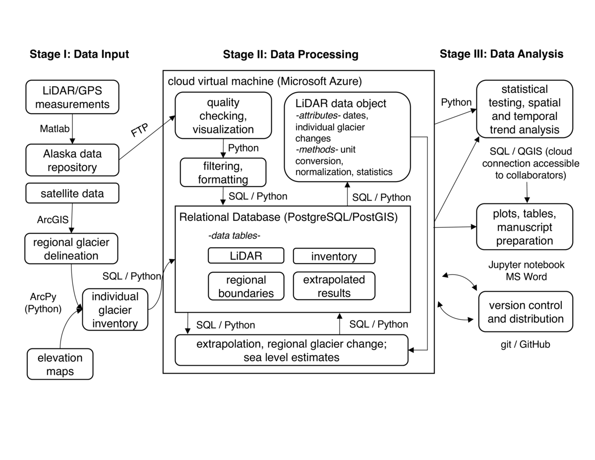 The workflow begins with annual field data collection that produces both GPS positional and LiDAR point cloud data, both in industry standard binary formats. Commercial proprietary software is used to process the data into four dimensional point observations (x, y, z and time), which are then further processed using Generic Mapping Tools (GMT) into gridded 10 m digital elevation models. These elevation maps are then subtracted from maps acquired at an earlier time to obtain a change in elevation along the flight line, using Matlab scripts. These results are stored in text files, with the file name describing the glacier name and start and end dates, and are located on a server at the University of Alaska Fairbanks. In a separate step, we assemble satellite imagery and regional digital elevation models for the Alaska region. We use ArcGIS, a commercial GIS software package, to manually digitize the glacier extent. ArcGIS provides a set of vector manipulation tools that enable our technicians to trace glacier outlines from satellite imagery. ArcGIS commands can also be scripted using the ArcPy library. We automate a series of GIS commands using ArcPy to calculate the distribution of glacier surface area with elevation for each of approximately 27,000 glaciers in Alaska.
The majority of our data processing and analysis occurs on a single Microsoft Azure Linux Virtual Machine (VM) that hosts a spatially enabled Relational Database (RDB). We find that hosting an RDB in the cloud is a core element of our reproducible workflow. Our RDB provides rapid query capabilities so that much of our spatial and temporal averaging can be carried out using efficient database algorithms. Our cloud hosting enables colleagues to make direct connections to the database to access spatial data using their local GIS software. We use the open source PostgreSQL database with the PostGIS extension, to which we ingest point, line and polygon geospatial datasets. Relevant tables include:
inventory: polygons of each glacier in Alaska with attributes of surface area, glacier type (whether terminating on land or ocean), name
regional boundaries: polygons of outlines of mountain ranges or climatic zones over which we perform regional extrapolations
LiDAR: measurements of elevation and volume changes on surveyed glaciers
extrapolated results: final estimates of the volume change of every glacier in Alaska
Each time we acquire new altimetry observations we run a Python script to connect via secure FTP to the server in Fairbanks and search for new text files across the directory structure. We use the Python Pandas library as an interface between our text file and RDB data objects. Specifically, once we ingest the data into a Pandas DataFrame, we can employ a series of methods to generate simple plots and export the data directly to our PostgreSQL database. We use similar Python tools to create and update the inventory and regional boundaries tables, for example to accommodate changes in surface area as glaciers retreat.
The LiDAR data object is the foundation of all subsequent processing and analysis. The data object is created via a function call with parameters describing a single or a regional grouping of glaciers. Each instance of the data object has predefined attributes enabling users to rapidly acquire elements of the raw data in the LiDAR table. For example, a user can issue a request to the LiDAR table for a specific glacier, returning a data object whose attributes contain that glacier's elevation change, area, and other statistical information. The data object also has several methods that handle the majority of the standard data processing and filtering workflow. These methods include algorithms that carry out unit conversions, normalize the data, calculate statistics and perform mass change calculations for each glacier. To perform these calculations we issue Structured Query Language (SQL) commands to the database from within our Python scripts.
In a final processing step, we utilize the grouping functionality of the LiDAR object methods to generate average elevation change profiles across glaciers grouped by type or by spatial location. For example, we found similar elevation change distributions across glaciers with similar terminus types (i.e. whether terminating in land or in water). Therefore we generated LiDAR objects averaged over type groupings, as queried from our inventory table, thereby returning a single estimate of elevation change versus elevation. In a final step, we invoked a function that regionally extrapolates these profiles to the unmeasured ice masses stored in the inventory table, based on their distribution of area with elevation. This returns a dictionary of ice mass changes by group, as well as an optional new database table containing mass change estimates for each of the 27,000 ice polygons in the region (table extrapolated results). All functions and methods run quickly, with the exception of steps involved in building extrapolated results, which takes about 15 minutes to run.
To analyze results and distribute our findings we host a permanent instance of a Jupyter notebook on our Linux VM and provide access to project team members. The notebooks, as well as the core Python scripts used to generate results, are also located in a GitHub repository. The notebook also contains markdown to provide metadata at each step in the analysis. Collaborators with experience writing SQL code can have direct access to the PostgreSQL database to perform their own queries. Other collaborators more familiar with GIS tools can connecting directly to the geospatially encoded tables to generate their own maps.
Pain points
Our team brought together researchers with different backgrounds and approaches to data handling and processing. The processing of raw LiDAR and GPS data is performed by a different group than the one handling the GIS and extrapolation portion of the project, and each uses different software tools. We dealt with this problem by creating standardized files at different stages of the processing chain. For example, the LiDAR/GPS team produced a stack of files processed to the point where they could be used for extrapolation, which were then ingested to the geospatial database. A challenge here is the data are replicated in multiple locations, requiring careful version control.
Another challenge is that some of our collaborators encountered problems when attempting to connect directly to our cloud computing resources. One issue is that Alaska has limited internet bandwidth so that transfer of data between Alaska and commercial cloud providers is slow. Another challenge is that many US government agencies have firewalls that restrict direct traffic with our cloud database services. Therefore our collaborators in government and/or those located in Alaska had to set up duplicate versions of our databases, creating challenges with version control and project management.
Key benefits
Our workflow provides a mechanism to continually update our analysis as new data arrive. Our project is funded for several more years, and we are now in a position to regenerate key figures and update sea level estimates every time we acquire new datasets. This will greatly diminish the time it takes for us to provide stakeholders with updated information on the status of Alaska glaciers and their contribution to sea level. Also, our data are uniquely dynamic, and must accommodate not only new data but changes to the base inventory as glacier geometries (area and elevation) change over time. By having all our inventory data in relational tables we can update individual polygons and account for the feedback effects of glacier area on mass balance.
Our workflow also provides a stable foundation that can accommodate changes in team composition over time. As students and technicians join and leave the project we can have them use and contribute to a repository of scripts, rather than having to reinvent things from scratch.
We are well positioned to explore our data in ways not previously possible. New collaborators are joining our team and making direct connections to our database, generating complex queries that are exploring what climatic and geometric factors may be driving the glacier mass changes we are observing in the field. Other similar LiDAR observation programs do not provide access to relational databases, limiting researchers' ability to perform spatial and temporal queries.
Key tools
Hosting our resources in a cloud environment played a vital role in making our workflow reproducible. The cloud enabled us to co-locate our scripts with the observations, enabling rapid processing and minimizing the need to transfer files. Additionally, using a relational database to store our geospatial datasets provided efficient methods for us to explore a wide range of spatial relationships in our datasets.
Questions
What does "reproducibility" mean to you?
Reproducibility is a crucial component of our workflow due to the dynamic nature of our monitoring campaign, and the need to constantly update the position and elevation of glaciers as they change in response to climate. We achieve reproducibility through:
Maintaining consistency in the input datasets
Utilizing a series of scripts to automate data ingest and filtering
Storing raw and filtered/processed data in a relational database
Generating data objects that handle typical data analysis functions
Scripting all manuscript figures in Jupyter notebooks
Why do you think that reproducibility in your domain is important?
Glaciology has become highly interdisciplinary in the past decade: oceanographers, climatologists, geodesists and glaciologists must integrate knowledge to close the sea level budget. Also, data from remote glacier regions is sparse, so any data we collect needs to be made available. By generating reproducible workflows we have a greater capacity to share information and to better understand exactly how each research team is processing their datasets.
How or where did you learn about reproducibility?
I learned these techniques through coursework, a visiting scientist appointment at Microsoft Research, and through self-directed learning.
What do you see as the major challenges to doing reproducible research in your domain, and do you have any suggestions?
The inability of non-specialists to make full use of our tools occasionally requires us to revert back to non-reproducible methods in order to get things done in a timely fashion. We are working to solve this problem by building lightweight Application Programming Interfaces enabling collaborators to access some of the core elements of our workflow through simple web protocols.
What do you view as the major incentives for doing reproducible research?
Within a research team, major incentives include: increased transparency in methods, increased accountability and ability to check for errors in processing, a reduction in spin-up time as new members join the team, and an ability to minimize duplication of effort. Between the team and other collaborators/stakeholders, we see major benefits in the ability to share and visualize results, and in our capacity to perform cross-disciplinary research.
Are there any best practices that you'd recommend for researchers in your field?
We recommend development and adherence to standards in geospatial data formats and distribution protocols.